>spectro(2018) was a friendly and informal contest for the best spectrogram generated with R code.
The spectrogram is a 2D/3D key visualisation tool for bioacoustics, ecoacoustics and other sound related disciplines. The spectrogram is not only useful for science, it can also be a nice graphical object with delicate shapes and colours.
The aim of this contest wass to share the beautiful sounds, R codes and spectrograms you may have in your files so that it can help others to produce nice graphics and figures.
But overall, the idea was to join science, fun, and maybe the arts!
The contest took place by the end of 2018. There international voting committee was composed of Fanny Rybak (France), Nadia Pieretti (Italy), Susan Fuller (Australia), Stefanie LaZerte (Canada), Tess Gridley (South Africa). The committee marked the anonymous submissions.
The prize was a printed sample of the book Sound analysis and synthesis with R for the winner, an electronic version of the same book for the second and the third, kindly offered by Springer, Berlin.
Please find below the winners and their submissions.
Congratulations to the winners and to all participants!
Xeno-Canto link
#-------------------------------------------
## LOADING REQUIRED PACKAGES
#-------------------------------------------
library(seewave)
library(tuneR)
library(ggplot2)
library(viridis)
library(grid)
library(gridExtra)
#-------------------------------------------
## SETUP FOR PLOTS
#-------------------------------------------
## PLOT LABELLERS
# x label formatter
s_formatter <- function(x){
lab <- paste0(x, " s")
}
# y label formatter
khz_formatter <- function(y){
lab <- paste0(y, " kHz")
}
## THEMES
oscillo_theme_dark <- theme(panel.grid.major.y = element_line(color="black", linetype = "dotted"),
panel.grid.major.x = element_blank(),
panel.grid.minor = element_blank(),
panel.background = element_rect(fill="transparent"),
panel.border = element_rect(linetype = "solid", fill = NA, color = "grey"),
axis.line = element_blank(),
legend.position = "none",
plot.background = element_rect(fill="black"),
plot.margin = unit(c(0,1,1,1), "lines"),
axis.title = element_blank(),
axis.text = element_text(size=14, color = "grey"),
axis.ticks = element_line(color="grey"))
hot_theme <- theme(panel.grid.major.y = element_line(color="black", linetype = "dotted"),
panel.grid.major.x = element_blank(),
panel.grid.minor = element_blank(),
panel.background = element_rect(fill="transparent"),
panel.border = element_rect(linetype = "solid", fill = NA, color = "grey"),
axis.line = element_blank(),
legend.position = "top",
legend.justification = "right",
legend.background = element_rect(fill="black"),
legend.key.width = unit(50, "native"),
legend.title = element_text(size=16, color="grey"),
legend.text = element_text(size=16, color="grey"),
plot.background = element_rect(fill="black"),
axis.title = element_blank(),
axis.text = element_text(size=16, color = "grey"),
axis.ticks = element_line(color="grey"))
hot_theme_grid <- theme(panel.grid.major.y = element_line(color="black", linetype = "dotted"),
panel.grid.major.x = element_blank(),
panel.grid.minor = element_blank(),
panel.background = element_rect(fill="transparent"),
panel.border = element_rect(linetype = "solid", fill = NA, color = "grey"),
axis.line = element_blank(),
legend.position = "top",
legend.justification = "right",
legend.background = element_rect(fill="black"),
legend.key.width = unit(50, "native"),
legend.title = element_text(size=16, color="grey"),
legend.text = element_text(size=16, color="grey"),
plot.background = element_rect(fill="black"),
plot.margin = margin(1,1,0,1, "lines"),
axis.title = element_blank(),
axis.text = element_text(size=16, color = "grey"),
axis.text.x = element_blank(),
axis.ticks = element_line(color="grey"))
## COLORS
hot_colors <- inferno(n=9)
#-------------------------------------------
## LOADING IN A WAV
#-------------------------------------------
# the path to .wav file
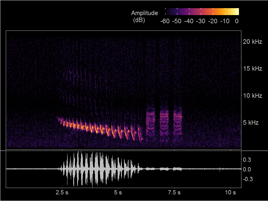
# note: the file is a clip of a canyon wren song, originally uploaded to xeno-canto.org by Bobby Wilcox
# note: the sound clip is in the creative commons (CC BY-NC-SA 4.0), downloaded from this link:
# https://www.xeno-canto.org/381415
wavefile_path <- ".\\XC381415 - Canyon Wren - Catherpes mexicanus.wav"
# loads a wave object from the .wav file path
wav <- readWave(wavefile_path)
# builds a dataframe of the wave object values
sample <- seq(1:length(wav@left))
time <- sample/wav@samp.rate
sample.left <- as.vector(cbind(wav@left))
df <- data.frame(sample, time, sample.left)
# subsets the dataframe to a more manageable size for plotting
last.index <- tail(df$sample,1)
index <- seq(from = 1, to = last.index, by = 20)
df2 <- df[index,]
#-------------------------------------------
## GGSPECTRO PLOTS
#-------------------------------------------
# builds a spectrogram using ggspectro()
# note: no x-axis labels because the plot is designed to be aligned with the oscillogram in a grid
# for x-axis labels, use hot_theme instead of hot_theme_grid
hotplot <- ggspectro(wave = wav, f = wav@samp.rate, ovlp=90)+
scale_x_continuous(labels=s_formatter, expand = c(0,0))+
scale_y_continuous(breaks = seq(from = 5, to = 20, by=5), expand = c(0,0), labels = khz_formatter, position = "right")+
geom_raster(aes(fill=amplitude), hjust = 0, vjust = 0, interpolate = F)+
scale_fill_gradientn(colours = hot_colors, name = "Amplitude \n (dB)", na.value = "transparent", limits = c(-60,0))+
hot_theme_grid
# builds an oscillogram
oscplot <- ggplot(df2)+
geom_line(mapping = aes(x=time, y=sample.left), color="grey")+
scale_x_continuous(labels=s_formatter, expand = c(0,0))+
scale_y_continuous(expand = c(0,0), position = "right")+
geom_hline(yintercept = 0, color="white", linetype = "dotted")+
oscillo_theme_dark
#-------------------------------------------
## PLOT GRID
#-------------------------------------------
gA=ggplot_gtable(ggplot_build(hotplot))
gB=ggplot_gtable(ggplot_build(oscplot))
maxWidth = grid::unit.pmax(gA$widths, gB$widths)
gA$widths <- as.list(maxWidth)
gB$widths <- as.list(maxWidth)
layo <- rbind(c(1,1,1),
c(1,1,1),
c(1,1,1),
c(2,2,2))
grid.newpage()
grid.arrange(gA, gB, layout_matrix = layo)
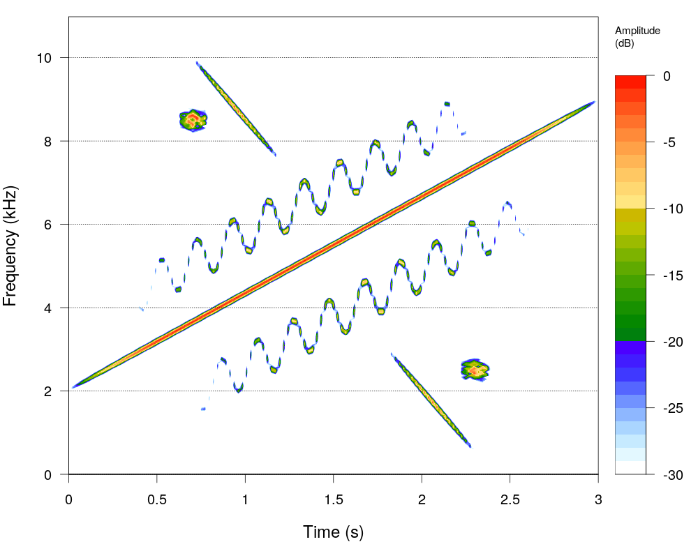
library(seewave)
f <- 22050

synth3 <- function(spectre, f, dephasage = TRUE, output = "Wave", complex = FALSE){
	  l <- length(spectre)
          phi <- runif(l)
          if(dephasage) {spectre <- spectre*exp(2*pi*1i*phi)}
          sound <- fft(spectre, inverse = TRUE)
          if (!complex) {sound <- Re(sound)}
          sound <- outputw(wave = sound, f = f, format = output)
          return(sound)
}

l0 <- 3*f

a0 <- synth(f, 3, 2000, a = 1, fm = c(0,0,(f-8000)/2,0,0), listen = FALSE, plot = FALSE, output = "matrix")
a <- a0*c(1:(l0/6),rep(f/2, l0 - l0/6 - ceiling(l0/6)),ceiling(l0/6):1)*2/f

b0 <- synth(f, 2, 4200, a = 0.5, shape = "sine", fm = c(500,5,(f-8000)/3,0,0,0), listen = FALSE, plot = FALSE, output = "matrix")
b <- c(rep(0,0.33*f),b0,rep(0,ceiling(0.67*f)))

c0 <- synth(f, 2, 1800, a = 0.5, shape = "sine", fm = c(500,5,(f-8000)/3,0,0,0), listen = FALSE, plot = FALSE, output= "matrix")
c <- c(rep(0,0.67*f),c0,rep(0,ceiling(0.33*f)))

l <- 0.18*f
variance <- 800

s <- exp(-(1:l-2500*l/f)^2/variance)
d0 <- synth3(s, f, dephasage = TRUE,output = "matrix",complex = FALSE)
d1 <- d0*(c(1:(l/2),(ceiling(l/2):1)))
d2 <- c(rep(0,ceiling(2.2*f)),d1,rep(0,l0-l-2.2*f))
d <- 2.5*d2/max(d2)

t <- exp(-(1:l-8512*l/f)^2/variance)
e0 <- synth3(t, f, dephasage = TRUE,output = "matrix",complex = FALSE)
e1 <- e0*(c(1:(l/2),(ceiling(l/2):1)))
e2 <- c(rep(0,l0-l-2.2*f),e1,rep(0,ceiling(2.2*f)))
e <- 2.5*e2/max(d2)

g0 <- synth(f,0.5,3000, a = 1, fm = c(0,0,-2500,0,0), shape = "tria", listen = FALSE, plot = FALSE,output="matrix")
g <- c(rep(0,1.8*f),g0,rep(0,ceiling(0.7*f)))

h0 <- synth(f,0.5,10025, a = 1, fm = c(0,0,-2500,0,0), shape = "tria", listen = FALSE, plot = FALSE,output="matrix")
h <- c(rep(0,ceiling(0.7*f)),h0,rep(0,1.8*f))

spectro(a+b+c+d+e+g+h,f)
listen(a+b+c+d+e+g+h,f)
Visit Braulio RG page
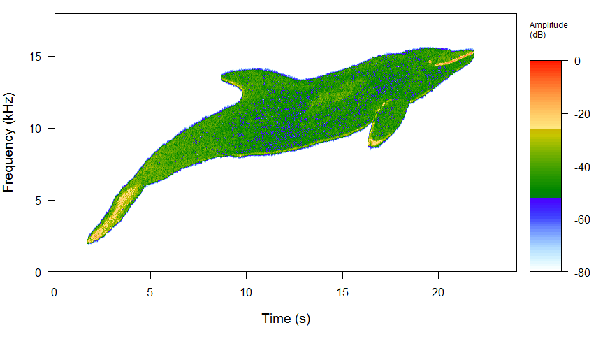
#load required packages#
library(seewave)
library(tuneR)
#load audio file in .wav#
tt=readWave("spectro2018_Braulio_Leon-Lopez.wav");
#built spectrogram#
spectro(tt, f=36000, wl=1024, wn="hanning", ovlp=50, collevels=seq(-80,0,1), palette= spectro.colors, grid=FALSE)