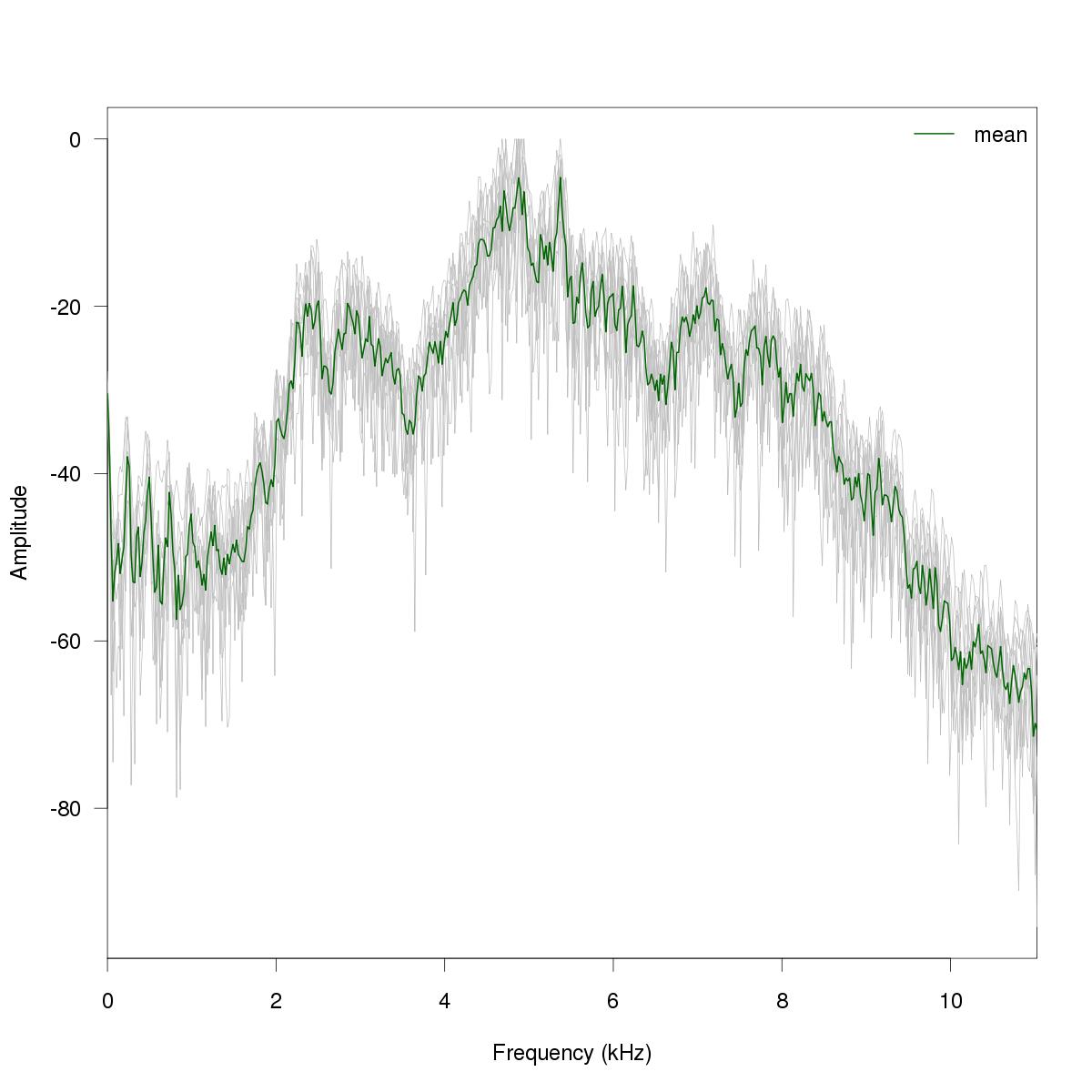
# a mean spectrum of 10 spectra computed at specific positions (pos) along the signal 
data(orni) 
pos <- c(0.04,0.07,0.2,0.23,0.34,0.37,0.48,0.5,0.62,0.64)
l <- length(pos)
wl <- 1024
m <- matrix(numeric(l*(wl/2)),nc=l)
for(i in 1:l) m[,i] <- spec(orni,f=22050,wl=wl,at=pos[i],dB=TRUE,plot=FALSE)[,2]
mean <- apply(m,MARGIN=1,mean)
x <- seq(0,11.025,length.out=nrow(m))
par(las=1)
matplot(x=x, y=m ,type="l", col="grey", lty=1, xlab="Frequency (kHz)", ylab="Amplitude", xaxs="i")
lines(x=x, y=mean, lwd=2, col="darkgreen")
legend("topright", legend="mean", lwd=2, col="darkgreen", bty="n")